Exercises-Chipotle 1

Ex2 - Getting and Knowing your Data

This time we are going to pull data directly from the internet. Special thanks to: https://github.com/justmarkham for sharing the dataset and materials.

Step 1. Import the necessary libraries

import pandas as pd
import numpy as np

Step 2. Import the dataset from this address.

Step 3. Assign it to a variable called chipo.

url = 'https://raw.githubusercontent.com/justmarkham/DAT8/master/data/chipotle.tsv'
chipo = pd.read_csv(url,sep='\t')

Step 4. See the first 10 entries

import pandas as pd
url ='https://raw.githubusercontent.com/justmarkham/DAT8/master/data/chipotle.tsv'
df = pd.read_csv(url,sep='\t')
df.head(10)

	order_id	quantity	item_name	choice_description	item_price
0	1	1	Chips and Fresh Tomato Salsa	NaN	$2.39
1	1	1	Izze	[Clementine]	$3.39
2	1	1	Nantucket Nectar	[Apple]	$3.39
3	1	1	Chips and Tomatillo-Green Chili Salsa	NaN	$2.39
4	2	2	Chicken Bowl	[Tomatillo-Red Chili Salsa (Hot), [Black Beans...	$16.98
5	3	1	Chicken Bowl	[Fresh Tomato Salsa (Mild), [Rice, Cheese, Sou...	$10.98
6	3	1	Side of Chips	NaN	$1.69
7	4	1	Steak Burrito	[Tomatillo Red Chili Salsa, [Fajita Vegetables...	$11.75
8	4	1	Steak Soft Tacos	[Tomatillo Green Chili Salsa, [Pinto Beans, Ch...	$9.25
9	5	1	Steak Burrito	[Fresh Tomato Salsa, [Rice, Black Beans, Pinto...	$9.25

Step 5. What is the number of observations in the dataset?

# Solution 1
row_count = len(df)
print(row_count)

# Solution 2
df.info()

<class 'pandas.core.frame.DataFrame'>
RangeIndex: 4622 entries, 0 to 4621
Data columns (total 5 columns):
 #   Column              Non-Null Count  Dtype 
---  ------              --------------  ----- 
 0   order_id            4622 non-null   int64 
 1   quantity            4622 non-null   int64 
 2   item_name           4622 non-null   object
 3   choice_description  3376 non-null   object
 4   item_price          4622 non-null   object
dtypes: int64(2), object(3)
memory usage: 180.7+ KB

Step 6. What is the number of columns in the dataset?

number_of_columns = len(df.columns)
print(number_of_columns)

Step 7. Print the name of all the columns.

df.columns

Index(['order_id', 'quantity', 'item_name', 'choice_description',
       'item_price'],
      dtype='object')

Step 8. How is the dataset indexed?

df.index

RangeIndex(start=0, stop=4622, step=1)

Step 9. Which was the most-ordered item?

data_sorted = df.groupby(["item_name"]).sum().sort_values(["quantity"],ascending=False)
max_value = data_sorted.head(1)
print(max_value)

              order_id  quantity  \
item_name                          
Chicken Bowl    713926       761   

                                             choice_description  \
item_name                                                         
Chicken Bowl  [Tomatillo-Red Chili Salsa (Hot), [Black Beans...   

                                                     item_price  
item_name                                                        
Chicken Bowl  $16.98 $10.98 $11.25 $8.75 $8.49 $11.25 $8.75 ...

Step 10. For the most-ordered item, how many items were ordered?

data_sorted = df.groupby(["item_name"]).sum().sort_values(["quantity"],ascending=False)
max_value = data_sorted.head(1)
print(max_value)

              order_id  quantity  \
item_name                          
Chicken Bowl    713926       761   

                                             choice_description  \
item_name                                                         
Chicken Bowl  [Tomatillo-Red Chili Salsa (Hot), [Black Beans...   

                                                     item_price  
item_name                                                        
Chicken Bowl  $16.98 $10.98 $11.25 $8.75 $8.49 $11.25 $8.75 ...

Step 11. What was the most ordered item in the choice_description column?

data_sorted = df.groupby(["choice_description"]).sum().sort_values(["quantity"],ascending=False)
max_value = data_sorted.head(1)
print(max_value)

                    order_id  quantity  \
choice_description                       
[Diet Coke]           123455       159   

                                                            item_name  \
choice_description                                                      
[Diet Coke]         Canned SodaCanned SodaCanned Soda6 Pack Soft D...   

                                                           item_price  
choice_description                                                     
[Diet Coke]         $2.18 $1.09 $1.09 $6.49 $2.18 $1.25 $1.09 $6.4...

Step 12. How many items were orderd in total?

total_sum_a = df['quantity'].sum()
print(total_sum_a)

Step 13. Turn the item price into a float

Step 13.a. Check the item price type

type_a = df['item_price'].dtype
print(type_a)

object

Step 13.b. Create a lambda function and change the type of item price

df['item_price'] = df['item_price'].apply(lambda x:x.replace('









# Exercises-chipotle 3





:::{.quarto-embed-nb-cell notebook="D:\code\jiedan\12-28\test\labs\Labexercises\Exercises-chipotle 3.ipynb" notebook-title="Visualizing Chipotle's Data" notebook-cellId="cell-0"}

# Visualizing Chipotle's Data

This time we are going to pull data directly from the internet.
Special thanks to: https://github.com/justmarkham for sharing the dataset and materials.

### Step 1. Import the necessary libraries

::: {#cell-2 .cell execution_count=13}
``` {.python .cell-code}
import pandas as pd
import matplotlib.pyplot as plt
from collections import Counter

# set this so the graphs open internally
%matplotlib inline

Step 2. Import the dataset from this address.

Step 3. Assign it to a variable called chipo.

chipo = pd.read_csv('https://raw.githubusercontent.com/justmarkham/DAT8/master/data/chipotle.tsv',sep='\t')
chipo

	order_id	quantity	item_name	choice_description	item_price
0	1	1	Chips and Fresh Tomato Salsa	NaN	$2.39
1	1	1	Izze	[Clementine]	$3.39
2	1	1	Nantucket Nectar	[Apple]	$3.39
3	1	1	Chips and Tomatillo-Green Chili Salsa	NaN	$2.39
4	2	2	Chicken Bowl	[Tomatillo-Red Chili Salsa (Hot), [Black Beans...	$16.98
...	...	...	...	...	...
4617	1833	1	Steak Burrito	[Fresh Tomato Salsa, [Rice, Black Beans, Sour ...	$11.75
4618	1833	1	Steak Burrito	[Fresh Tomato Salsa, [Rice, Sour Cream, Cheese...	$11.75
4619	1834	1	Chicken Salad Bowl	[Fresh Tomato Salsa, [Fajita Vegetables, Pinto...	$11.25
4620	1834	1	Chicken Salad Bowl	[Fresh Tomato Salsa, [Fajita Vegetables, Lettu...	$8.75
4621	1834	1	Chicken Salad Bowl	[Fresh Tomato Salsa, [Fajita Vegetables, Pinto...	$8.75

4622 rows × 5 columns

Step 4. See the first 10 entries

chipo.head(10)

	order_id	quantity	item_name	choice_description	item_price
0	1	1	Chips and Fresh Tomato Salsa	NaN	2.39
1	1	1	Izze	[Clementine]	3.39
2	1	1	Nantucket Nectar	[Apple]	3.39
3	1	1	Chips and Tomatillo-Green Chili Salsa	NaN	2.39
4	2	2	Chicken Bowl	[Tomatillo-Red Chili Salsa (Hot), [Black Beans...	16.98
5	3	1	Chicken Bowl	[Fresh Tomato Salsa (Mild), [Rice, Cheese, Sou...	10.98
6	3	1	Side of Chips	NaN	1.69
7	4	1	Steak Burrito	[Tomatillo Red Chili Salsa, [Fajita Vegetables...	11.75
8	4	1	Steak Soft Tacos	[Tomatillo Green Chili Salsa, [Pinto Beans, Ch...	9.25
9	5	1	Steak Burrito	[Fresh Tomato Salsa, [Rice, Black Beans, Pinto...	9.25

Step 5. Create a histogram of the top 5 items bought

# get the Series of the names
x = chipo.item_name

# use the Counter class from collections to create a dictionary with keys(text) and frequency
letter_counts = Counter(x)

# convert the dictionary to a DataFrame
df = pd.DataFrame.from_dict(letter_counts, orient='index')

# sort the values from the top to the least value and slice the first 5 items
df = df[0].sort_values(ascending = True)[45:50]

# create the plot
df.plot(kind='bar')

# Set the title and labels
plt.xlabel('Items')
plt.ylabel('Number of Times Ordered')
plt.title('Most ordered Chipotle\'s Items')

# show the plot
plt.show()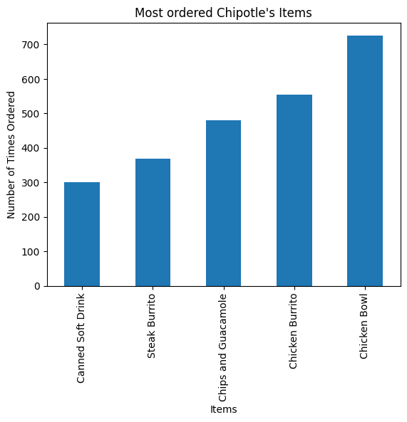

Step 6. Create a scatterplot with the number of items orderered per order price

Hint: Price should be in the X-axis and Items ordered in the Y-axis

# create a list of prices
chipo.item_price = [float(value[1:-1]) for value in chipo.item_price] # strip the dollar sign and trailing space

# then groupby the orders and sum
orders = chipo.groupby('order_id').sum()

# creates the scatterplot
# plt.scatter(orders.quantity, orders.item_price, s = 50, c = 'green')
plt.scatter(x = orders.item_price, y = orders.quantity, s = 50, c = 'green')

# Set the title and labels
plt.xlabel('Order Price')
plt.ylabel('Items ordered')
plt.title('Number of items ordered per order price')
plt.ylim(0)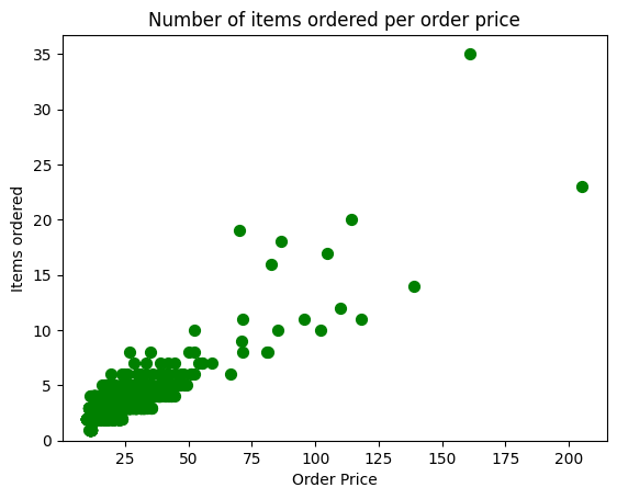

Step 7. BONUS: Create a question and a graph to answer your own question.

# 用柱形图显示商品销售额前10的商品
def parse_price(price):
    return float(price[1:])

item_price_new = chipo['item_price'].apply(parse_price)
chipo['item_price_new']=item_price_new

a = chipo.groupby('item_name')['item_price_new'].sum()
b = a.sort_values(ascending=False)

b.head(10).plot(kind='bar' , figsize=(10,5))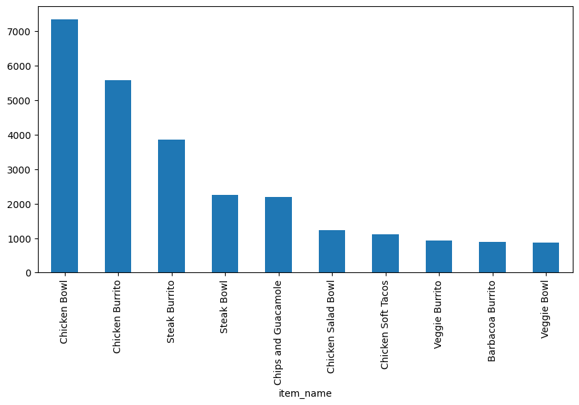

Source: Ex2 - Getting and Knowing your Data

Exercises-Occupation 1

Ex3 - Getting and Knowing your Data

This time we are going to pull data directly from the internet. Special thanks to: https://github.com/justmarkham for sharing the dataset and materials.

Step 1. Import the necessary libraries

import pandas as pd

Step 2. Import the dataset from this address.

Step 3. Assign it to a variable called users and use the ‘user_id’ as index

users = pd.read_csv('https://raw.githubusercontent.com/justmarkham/DAT8/master/data/u.user', 
                      sep='|', index_col='user_id')

Step 4. See the first 25 entries

users.head(25)

	age	gender	occupation	zip_code
user_id
1	24	M	technician	85711
2	53	F	other	94043
3	23	M	writer	32067
4	24	M	technician	43537
5	33	F	other	15213
6	42	M	executive	98101
7	57	M	administrator	91344
8	36	M	administrator	05201
9	29	M	student	01002
10	53	M	lawyer	90703
11	39	F	other	30329
12	28	F	other	06405
13	47	M	educator	29206
14	45	M	scientist	55106
15	49	F	educator	97301
16	21	M	entertainment	10309
17	30	M	programmer	06355
18	35	F	other	37212
19	40	M	librarian	02138
20	42	F	homemaker	95660
21	26	M	writer	30068
22	25	M	writer	40206
23	30	F	artist	48197
24	21	F	artist	94533
25	39	M	engineer	55107

Step 5. See the last 10 entries

users.tail(10)

	age	gender	occupation	zip_code
user_id
934	61	M	engineer	22902
935	42	M	doctor	66221
936	24	M	other	32789
937	48	M	educator	98072
938	38	F	technician	55038
939	26	F	student	33319
940	32	M	administrator	02215
941	20	M	student	97229
942	48	F	librarian	78209
943	22	M	student	77841

Step 6. What is the number of observations in the dataset?

users.shape[0]

Step 7. What is the number of columns in the dataset?

users.shape[1]

Step 8. Print the name of all the columns.

users.columns

Index(['age', 'gender', 'occupation', 'zip_code'], dtype='object')

Step 9. How is the dataset indexed?

# "the index" (aka "the labels")    
# 【索引，又被称为标签】
users.index

Index([  1,   2,   3,   4,   5,   6,   7,   8,   9,  10,
       ...
       934, 935, 936, 937, 938, 939, 940, 941, 942, 943],
      dtype='int64', name='user_id', length=943)

Step 10. What is the data type of each column?

users.dtypes

age            int64
gender        object
occupation    object
zip_code      object
dtype: object

Step 11. Print only the occupation column

users.occupation

#or

users['occupation']

user_id
1         technician
2              other
3             writer
4         technician
5              other
           ...      
939          student
940    administrator
941          student
942        librarian
943          student
Name: occupation, Length: 943, dtype: object

Step 12. How many different occupations are in this dataset?

users.occupation.nunique()
#or by using value_counts() which returns the count of unique elements
#users.occupation.value_counts().count()

Step 13. What is the most frequent occupation?

#Because "most" is asked
users.occupation.value_counts().head(1).index[0]

#or
#to have the top 5

# users.occupation.value_counts().head()

'student'

Step 14. Summarize the DataFrame.

users.describe() #Notice: by default, only the numeric columns are returned.

	age
count	943.000000
mean	34.051962
std	12.192740
min	7.000000
25%	25.000000
50%	31.000000
75%	43.000000
max	73.000000

Step 15. Summarize all the columns

users.describe(include = "all") #Notice: By default, only the numeric columns are returned.

	age	gender	occupation	zip_code
count	943.000000	943	943	943
unique	NaN	2	21	795
top	NaN	M	student	55414
freq	NaN	670	196	9
mean	34.051962	NaN	NaN	NaN
std	12.192740	NaN	NaN	NaN
min	7.000000	NaN	NaN	NaN
25%	25.000000	NaN	NaN	NaN
50%	31.000000	NaN	NaN	NaN
75%	43.000000	NaN	NaN	NaN
max	73.000000	NaN	NaN	NaN

Step 16. Summarize only the occupation column

users.occupation.describe()

count         943
unique         21
top       student
freq          196
Name: occupation, dtype: object

Step 17. What is the mean age of users?

round(users.age.mean())

Step 18. What is the age with least occurrence?

users.age.value_counts().tail() #7, 10, 11, 66 and 73 years -> only 1 occurrence

age
7     1
66    1
11    1
10    1
73    1
Name: count, dtype: int64

Source: Ex3 - Getting and Knowing your Data

Exercises-World Food Facts 1

Exercise 1

Step 1. Go to https://www.kaggle.com/openfoodfacts/world-food-facts/data

Step 2. Download the dataset to your computer and unzip it.

Step 3. Use the tsv file and assign it to a dataframe called food

import pandas as pd
import numpy as np
food = pd.read_csv('en.openfoodfacts.org.products.tsv',sep='\t')

Step 4. See the first 5 entries

food.head()

	code	url	creator	created_t	created_datetime	last_modified_t	last_modified_datetime	product_name	generic_name	quantity	...	fruits-vegetables-nuts_100g	fruits-vegetables-nuts-estimate_100g	collagen-meat-protein-ratio_100g	cocoa_100g	chlorophyl_100g	carbon-footprint_100g	nutrition-score-fr_100g	nutrition-score-uk_100g	glycemic-index_100g	water-hardness_100g
0	3087	http://world-en.openfoodfacts.org/product/0000...	openfoodfacts-contributors	1474103866	2016-09-17T09:17:46Z	1474103893	2016-09-17T09:18:13Z	Farine de blé noir	NaN	1kg	...	NaN	NaN	NaN	NaN	NaN	NaN	NaN	NaN	NaN	NaN
1	4530	http://world-en.openfoodfacts.org/product/0000...	usda-ndb-import	1489069957	2017-03-09T14:32:37Z	1489069957	2017-03-09T14:32:37Z	Banana Chips Sweetened (Whole)	NaN	NaN	...	NaN	NaN	NaN	NaN	NaN	NaN	14.0	14.0	NaN	NaN
2	4559	http://world-en.openfoodfacts.org/product/0000...	usda-ndb-import	1489069957	2017-03-09T14:32:37Z	1489069957	2017-03-09T14:32:37Z	Peanuts	NaN	NaN	...	NaN	NaN	NaN	NaN	NaN	NaN	0.0	0.0	NaN	NaN
3	16087	http://world-en.openfoodfacts.org/product/0000...	usda-ndb-import	1489055731	2017-03-09T10:35:31Z	1489055731	2017-03-09T10:35:31Z	Organic Salted Nut Mix	NaN	NaN	...	NaN	NaN	NaN	NaN	NaN	NaN	12.0	12.0	NaN	NaN
4	16094	http://world-en.openfoodfacts.org/product/0000...	usda-ndb-import	1489055653	2017-03-09T10:34:13Z	1489055653	2017-03-09T10:34:13Z	Organic Polenta	NaN	NaN	...	NaN	NaN	NaN	NaN	NaN	NaN	NaN	NaN	NaN	NaN

5 rows × 163 columns

Step 5. What is the number of observations in the dataset?

food.shape[0]

Step 6. What is the number of columns in the dataset?

food.shape[1]
food.info()

<class 'pandas.core.frame.DataFrame'>
RangeIndex: 356027 entries, 0 to 356026
Columns: 163 entries, code to water-hardness_100g
dtypes: float64(107), object(56)
memory usage: 442.8+ MB

Step 7. Print the name of all the columns.

food.columns

Index(['code', 'url', 'creator', 'created_t', 'created_datetime',
       'last_modified_t', 'last_modified_datetime', 'product_name',
       'generic_name', 'quantity',
       ...
       'fruits-vegetables-nuts_100g', 'fruits-vegetables-nuts-estimate_100g',
       'collagen-meat-protein-ratio_100g', 'cocoa_100g', 'chlorophyl_100g',
       'carbon-footprint_100g', 'nutrition-score-fr_100g',
       'nutrition-score-uk_100g', 'glycemic-index_100g',
       'water-hardness_100g'],
      dtype='object', length=163)

Step 8. What is the name of 105th column?

food.columns[104]

'-glucose_100g'

Step 9. What is the type of the observations of the 105th column?

food.dtypes[food.columns[104]]

dtype('float64')

Step 10. How is the dataset indexed?

food.index

RangeIndex(start=0, stop=356027, step=1)

Step 11. What is the product name of the 19th observation?

food.values[18][7]

'Lotus Organic Brown Jasmine Rice'

Source: Exercise 1

77fba8e3b056425013930abb11e0a970

import pandas as pd
import matplotlib as mpl
import matplotlib.pyplot as plt
import numpy as np
from pathlib import Path
from lets_plot import *


LetsPlot.setup_html(no_js=True)

plt.style.use(

    "https://raw.githubusercontent.com/aeturrell/core_python/main/plot_style.txt"
)

data_np = pd.read_excel(
    "data/doing-economics-datafile-working-in-excel-project-2.xlsx",
    usecols="A:Q",
    header=1,
    index_col="Period",
)
data_n = data_np.iloc[:10, :].copy()
data_p = data_np.iloc[14:24, :].copy()

test_data = {
    "City A": [14.1, 14.1, 13.7],
    "City B": [11.0, 12.6, 12.1],
}


# Original dataframe
test_df = pd.DataFrame.from_dict(test_data)
# A copy of the dataframe
test_copy = test_df.copy()
# A pointer to the dataframe
test_pointer = test_df


test_pointer.iloc[1, 1] = 99

print("test_df=")
print(f"{test_df}\n")
print("test_copy=")
print(f"{test_copy}\n")

test_df=
   City A  City B
0    14.1    11.0
1    14.1    99.0
2    13.7    12.1

test_copy=
   City A  City B
0    14.1    11.0
1    14.1    12.6
2    13.7    12.1

data_n.info()

<class 'pandas.core.frame.DataFrame'>
Index: 10 entries, 1 to 10
Data columns (total 16 columns):
 #   Column           Non-Null Count  Dtype 
---  ------           --------------  ----- 
 0   Copenhagen       10 non-null     object
 1   Dnipropetrovs’k  10 non-null     object
 2   Minsk            10 non-null     object
 3   St. Gallen       10 non-null     object
 4   Muscat           10 non-null     object
 5   Samara           10 non-null     object
 6   Zurich           10 non-null     object
 7   Boston           10 non-null     object
 8   Bonn             10 non-null     object
 9   Chengdu          10 non-null     object
 10  Seoul            10 non-null     object
 11  Riyadh           10 non-null     object
 12  Nottingham       10 non-null     object
 13  Athens           10 non-null     object
 14  Istanbul         10 non-null     object
 15  Melbourne        10 non-null     object
dtypes: object(16)
memory usage: 1.3+ KB

data_n = data_n.astype("double")
data_p = data_p.astype("double")

mean_n_c = data_n.mean(axis=1)
mean_p_c = data_p.agg(np.mean, axis=1)

fig, ax = plt.subplots()
mean_n_c.plot(ax=ax, label="Without punishment")
mean_p_c.plot(ax=ax, label="With punishment")
ax.set_title("Average contributions to the public goods game")
ax.set_ylabel("Average contribution")
ax.legend();

partial_names_list = ["F. Kennedy", "Lennon", "Maynard Keynes", "Wayne"]
["John " + name for name in partial_names_list]

['John F. Kennedy', 'John Lennon', 'John Maynard Keynes', 'John Wayne']

# Create new dataframe with bars in
compare_grps = pd.DataFrame(
    [mean_n_c.loc[[1, 10]], mean_p_c.loc[[1, 10]]],
    index=["Without punishment", "With punishment"],
)
# Rename columns to have 'round' in them
compare_grps.columns = ["Round " + str(i) for i in compare_grps.columns]
# Swap the column and index variables around with the transpose function, ready for plotting (.T is transpose)
compare_grps = compare_grps.T
# Make a bar chart
compare_grps.plot.bar(rot=0);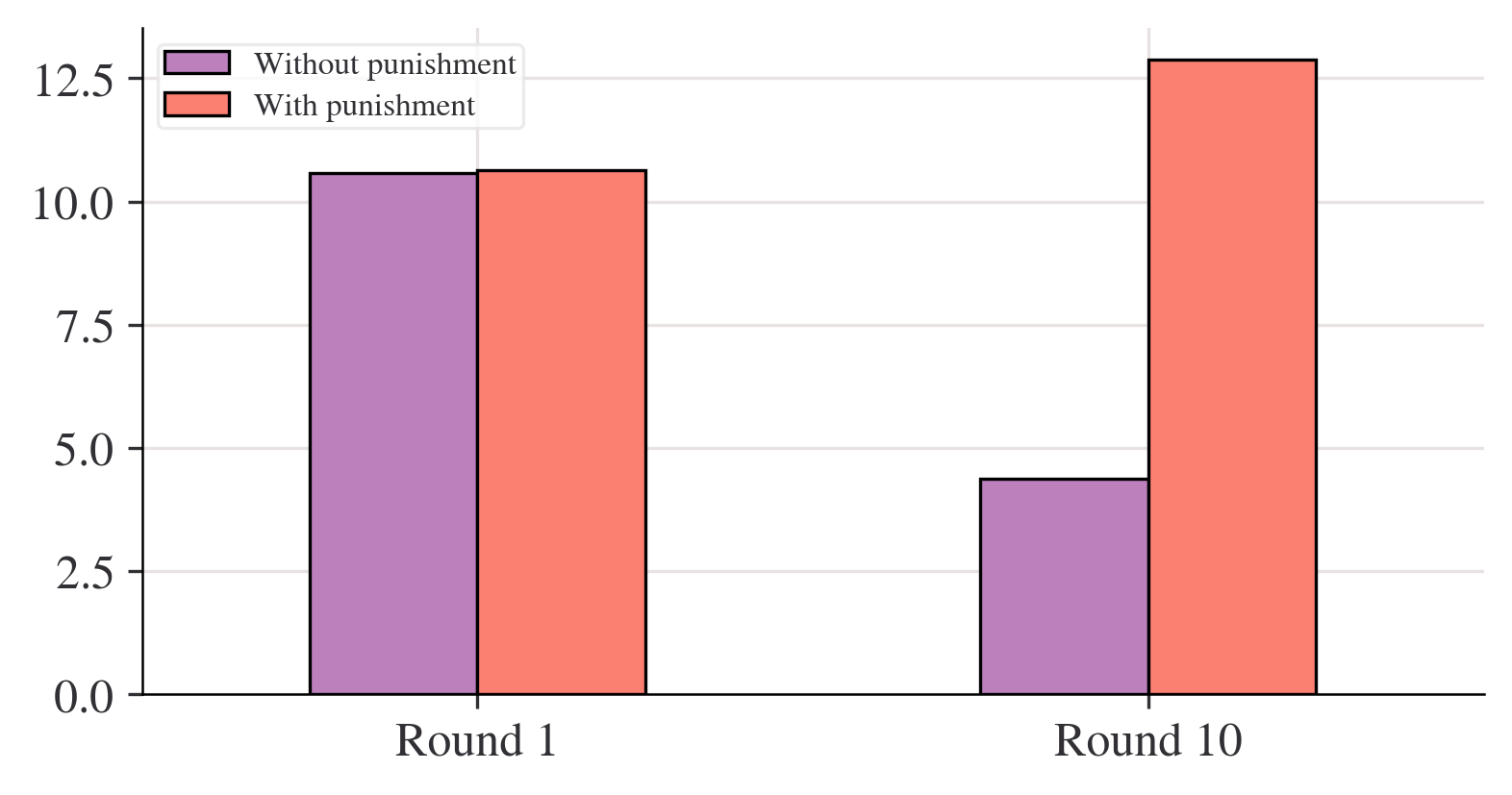

n_c = data_n.agg(["std", "var", "mean"], 1)
n_c

	std	var	mean
Period
1	2.020724	4.083325	10.578313
2	2.238129	5.009220	10.628398
3	2.329569	5.426891	10.407079
4	2.068213	4.277504	9.813033
5	2.108329	4.445049	9.305433
6	2.240881	5.021549	8.454844
7	2.136614	4.565117	7.837568
8	2.349442	5.519880	7.376388
9	2.413845	5.826645	6.392985
10	2.187126	4.783520	4.383769

p_c = data_p.agg(["std", "var", "mean"], 1)

fig, ax = plt.subplots()
n_c["mean"].plot(ax=ax, label="mean")
# mean + 2 standard deviations
(n_c["mean"] + 2 * n_c["std"]).plot(ax=ax, ylim=(0, None), color="red", label="±2 s.d.")
# mean - 2 standard deviations
(n_c["mean"] - 2 * n_c["std"]).plot(ax=ax, ylim=(0, None), color="red", label="")
for i in range(len(data_n.columns)):
    ax.scatter(x=data_n.index, y=data_n.iloc[:, i], color="k", alpha=0.3)
ax.legend()
ax.set_ylabel("Average contribution")
ax.set_title("Contribution to public goods game without punishment")
plt.show();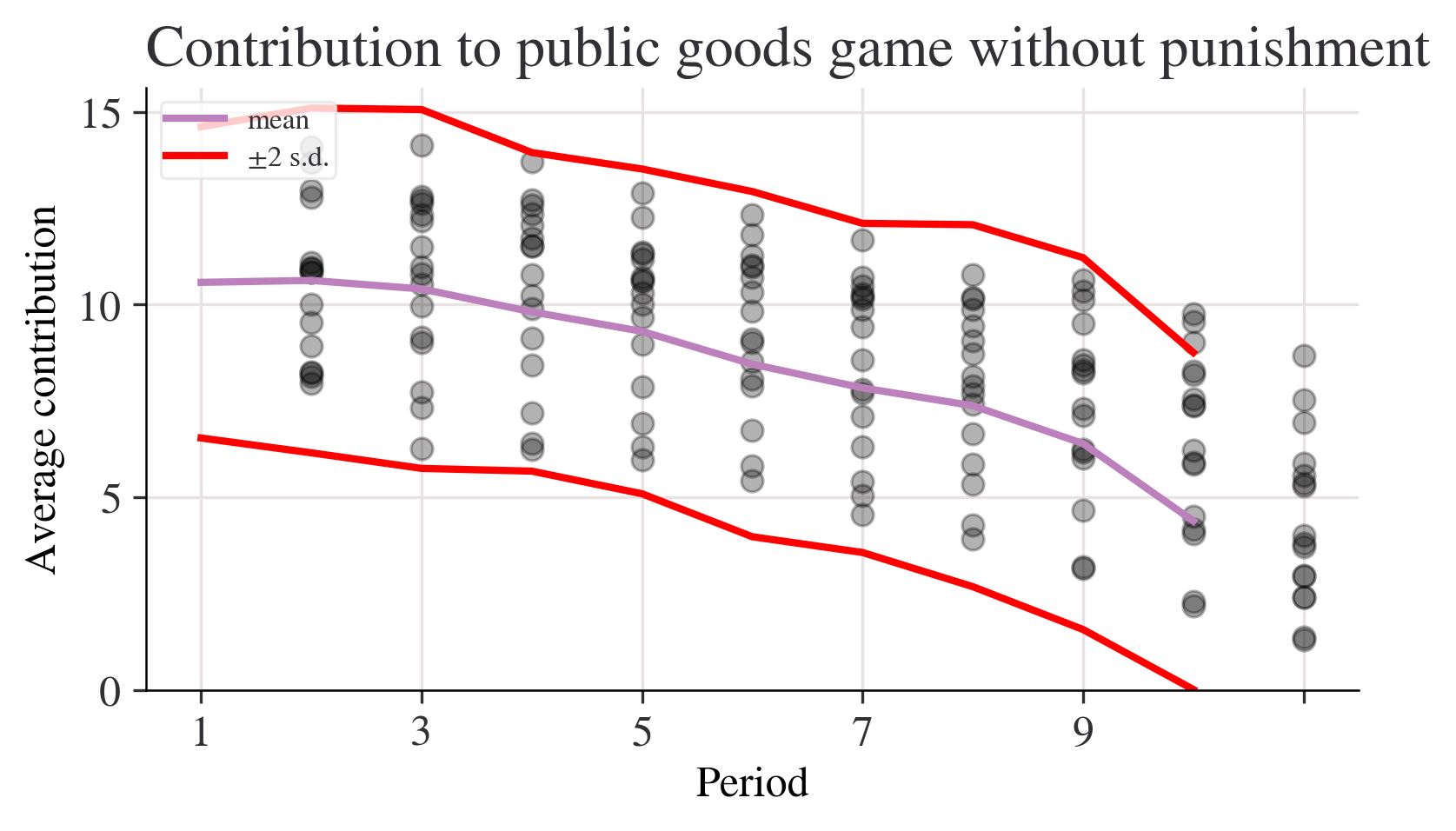

fig, ax = plt.subplots()
p_c["mean"].plot(ax=ax, label="mean")
# mean + 2 sd
(p_c["mean"] + 2 * p_c["std"]).plot(ax=ax, ylim=(0, None), color="red", label="±2 s.d.")
# mean - 2 sd
(p_c["mean"] - 2 * p_c["std"]).plot(ax=ax, ylim=(0, None), color="red", label="")
for i in range(len(data_p.columns)):
    ax.scatter(x=data_p.index, y=data_p.iloc[:, i], color="k", alpha=0.3)
ax.legend()
ax.set_ylabel("Average contribution")
ax.set_title("Contribution to public goods game with punishment")
plt.show();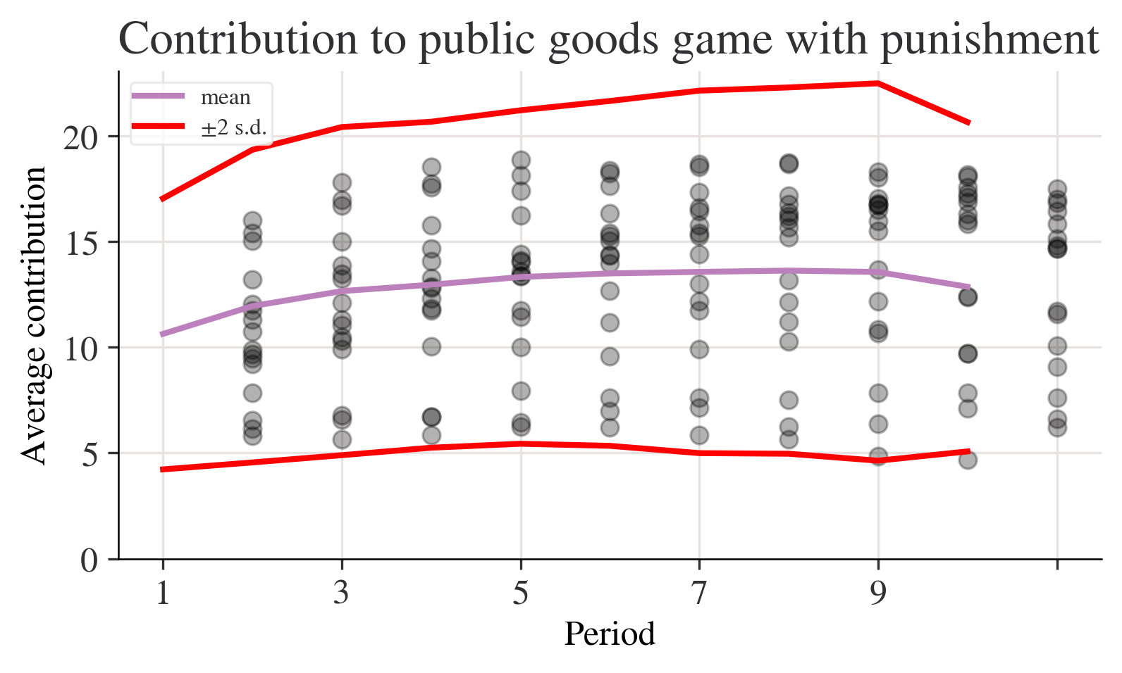

data_p.apply(lambda x: x.max() - x.min(), axis=1)

Period
1     10.199675
2     12.185065
3     12.689935
4     12.625000
5     12.140375
6     12.827541
7     13.098931
8     13.482621
9     13.496754
10    11.307360
dtype: float64

# A lambda function accepting three inputs, a, b, and c, and calculating the sum of the squares
test_function = lambda a, b, c: a**2 + b**2 + c**2


# Now we apply the function by handing over (in parenthesis) the following inputs: a=3, b=4 and c=5
test_function(3, 4, 5)

range_function = lambda x: x.max() - x.min()
range_p = data_p.apply(range_function, axis=1)
range_n = data_n.apply(range_function, axis=1)

fig, ax = plt.subplots()
range_p.plot(ax=ax, label="With punishment")
range_n.plot(ax=ax, label="Without punishment")
ax.set_ylim(0, None)
ax.legend()
ax.set_title("Range of contributions to the public goods game")
plt.show();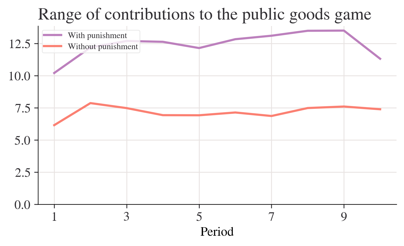

funcs_to_apply = [range_function, "max", "min", "std", "mean"]
summ_p = data_p.apply(funcs_to_apply, axis=1).rename(columns={"<lambda>": "range"})
summ_n = data_n.apply(funcs_to_apply, axis=1).rename(columns={"<lambda>": "range"})

summ_n.loc[[1, 10], :].round(2)

	range	max	min	std	mean
Period
1	6.14	14.10	7.96	2.02	10.58
10	7.38	8.68	1.30	2.19	4.38

summ_p.loc[[1, 10], :].round(2)

	range	max	min	std	mean
Period
1	10.20	16.02	5.82	3.21	10.64
10	11.31	17.51	6.20	3.90	12.87

%pip install pingouin

Collecting pingouin
  Downloading pingouin-0.5.5-py3-none-any.whl.metadata (19 kB)
Requirement already satisfied: matplotlib in c:\users\hp\anaconda3\lib\site-packages (from pingouin) (3.9.2)
Requirement already satisfied: numpy in c:\users\hp\anaconda3\lib\site-packages (from pingouin) (1.26.4)
Requirement already satisfied: pandas>=1.5 in c:\users\hp\anaconda3\lib\site-packages (from pingouin) (2.2.2)
Collecting pandas-flavor (from pingouin)
  Downloading pandas_flavor-0.6.0-py3-none-any.whl.metadata (6.3 kB)
Requirement already satisfied: scikit-learn>=1.2 in c:\users\hp\anaconda3\lib\site-packages (from pingouin) (1.5.1)
Requirement already satisfied: scipy in c:\users\hp\anaconda3\lib\site-packages (from pingouin) (1.13.1)
Requirement already satisfied: seaborn in c:\users\hp\anaconda3\lib\site-packages (from pingouin) (0.13.2)
Requirement already satisfied: statsmodels in c:\users\hp\anaconda3\lib\site-packages (from pingouin) (0.14.2)
Requirement already satisfied: tabulate in c:\users\hp\anaconda3\lib\site-packages (from pingouin) (0.9.0)
Requirement already satisfied: python-dateutil>=2.8.2 in c:\users\hp\anaconda3\lib\site-packages (from pandas>=1.5->pingouin) (2.9.0.post0)
Requirement already satisfied: pytz>=2020.1 in c:\users\hp\anaconda3\lib\site-packages (from pandas>=1.5->pingouin) (2024.1)
Requirement already satisfied: tzdata>=2022.7 in c:\users\hp\anaconda3\lib\site-packages (from pandas>=1.5->pingouin) (2023.3)
Requirement already satisfied: joblib>=1.2.0 in c:\users\hp\anaconda3\lib\site-packages (from scikit-learn>=1.2->pingouin) (1.4.2)
Requirement already satisfied: threadpoolctl>=3.1.0 in c:\users\hp\anaconda3\lib\site-packages (from scikit-learn>=1.2->pingouin) (3.5.0)
Requirement already satisfied: contourpy>=1.0.1 in c:\users\hp\anaconda3\lib\site-packages (from matplotlib->pingouin) (1.2.0)
Requirement already satisfied: cycler>=0.10 in c:\users\hp\anaconda3\lib\site-packages (from matplotlib->pingouin) (0.11.0)
Requirement already satisfied: fonttools>=4.22.0 in c:\users\hp\anaconda3\lib\site-packages (from matplotlib->pingouin) (4.51.0)
Requirement already satisfied: kiwisolver>=1.3.1 in c:\users\hp\anaconda3\lib\site-packages (from matplotlib->pingouin) (1.4.4)
Requirement already satisfied: packaging>=20.0 in c:\users\hp\anaconda3\lib\site-packages (from matplotlib->pingouin) (24.1)
Requirement already satisfied: pillow>=8 in c:\users\hp\anaconda3\lib\site-packages (from matplotlib->pingouin) (10.4.0)
Requirement already satisfied: pyparsing>=2.3.1 in c:\users\hp\anaconda3\lib\site-packages (from matplotlib->pingouin) (3.1.2)
Requirement already satisfied: xarray in c:\users\hp\anaconda3\lib\site-packages (from pandas-flavor->pingouin) (2023.6.0)
Requirement already satisfied: patsy>=0.5.6 in c:\users\hp\anaconda3\lib\site-packages (from statsmodels->pingouin) (0.5.6)
Requirement already satisfied: six in c:\users\hp\anaconda3\lib\site-packages (from patsy>=0.5.6->statsmodels->pingouin) (1.16.0)
Downloading pingouin-0.5.5-py3-none-any.whl (204 kB)
Downloading pandas_flavor-0.6.0-py3-none-any.whl (7.2 kB)
Installing collected packages: pandas-flavor, pingouin
Successfully installed pandas-flavor-0.6.0 pingouin-0.5.5
Note: you may need to restart the kernel to use updated packages.

import pingouin as pg

pg.ttest(x=data_n.iloc[0, :], y=data_p.iloc[0, :])

	T	dof	alternative	p-val	CI95%	cohen-d	BF10	power
T-test	-0.063782	30	two-sided	0.949567	[-2.0, 1.87]	0.02255	0.337	0.050437

pg.ttest(x=data_n.iloc[0, :], y=data_p.iloc[0, :], paired=True)

	T	dof	alternative	p-val	CI95%	cohen-d	BF10	power
T-test	-0.149959	15	two-sided	0.882795	[-0.92, 0.8]	0.02255	0.258	0.05082

Source: Original dataframe

4.IMDb and Douban top-250 movie datasets

import pandas as pd
import matplotlib.pyplot as plt
import seaborn as sns

imdb_data = pd.read_csv('IMDB_Top250.csv')  # Replace with actual file path
douban_data = pd.read_csv('douban_top250.csv')  # Replace with actual file path

from bs4 import BeautifulSoup
import re
import urllib.request, urllib.error  # for URL requests
import csv  # for saving as CSV

# Regular expressions to extract information
findLink = re.compile(r'<a href="(.*?)">')  # detail link
findImgSrc = re.compile(r'<img.*src="(.*?)"', re.S)  # image link
findTitle = re.compile(r'<span class="title">(.*)</span>')  # movie title
findRating = re.compile(r'<span class="rating_num" property="v:average">(.*)</span>')  # rating
findJudge = re.compile(r'<span>(\d*)人评价</span>')  # number of reviews
findInq = re.compile(r'<span class="inq">(.*)</span>')  # summary
findBd = re.compile(r'<p class="">(.*?)</p>', re.S)  # additional info

import pandas as pd
import matplotlib.pyplot as plt

# Load datasets
douban_file_path = 'douban_top250.csv'  
imdb_file_path = 'IMDB_Top250.csv'      

douban_data = pd.read_csv(douban_file_path, encoding='utf-8', on_bad_lines='skip')
imdb_data = pd.read_csv(imdb_file_path, encoding='utf-8', on_bad_lines='skip')

# Renaming columns for clarity and merging compatibility
douban_data.rename(columns={
    '影片中文名': 'Title',
    '评分': 'Douban_Score',
    '评价数': 'Douban_Reviews',
    '相关信息': 'Douban_Info'
}, inplace=True)

imdb_data.rename(columns={
    'Name': 'Title',
    'Year': 'Release_Year',
    'IMDB Ranking': 'IMDB_Score',
    'Genre': 'IMDB_Genre',
    'Director': 'IMDB_Director'
}, inplace=True)

# Calculate average scores for both platforms
douban_avg_score = douban_data['Douban_Score'].mean()
imdb_avg_score = imdb_data['IMDB_Score'].mean()

# Find overlapping movies by title
overlap_movies = pd.merge(douban_data, imdb_data, on='Title')

# Visualize average scores
plt.figure(figsize=(8, 5))
plt.bar(['Douban', 'IMDb'], [douban_avg_score, imdb_avg_score], alpha=0.7)
plt.title('Average Scores: Douban vs IMDb')
plt.ylabel('Average Score')
plt.show()

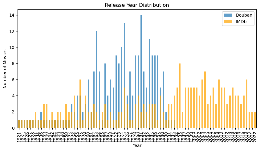
# Analyze release year distribution
plt.figure(figsize=(10, 5))
douban_data['Douban_Info'] = douban_data['Douban_Info'].astype(str)
douban_years = douban_data['Douban_Info'].str.extract(r'(\d{4})').dropna()
douban_years = douban_years[0].astype(int).value_counts().sort_index()

imdb_years = imdb_data['Release_Year'].value_counts().sort_index()

douban_years.plot(kind='bar', alpha=0.7, label='Douban', figsize=(10, 5))
imdb_years.plot(kind='bar', alpha=0.7, label='IMDb', color='orange')
plt.title('Release Year Distribution')
plt.xlabel('Year')
plt.ylabel('Number of Movies')
plt.legend()
plt.show()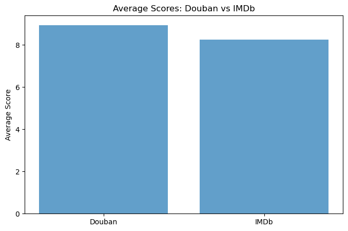

# Analyze genre distribution
imdb_genres = imdb_data['IMDB_Genre'].str.split(',').explode().str.strip().value_counts()
plt.figure(figsize=(10, 5))
imdb_genres.head(10).plot(kind='bar', alpha=0.7, color='orange')
plt.title('Top 10 IMDb Genres')
plt.xlabel('Genre')
plt.ylabel('Count')
plt.show()

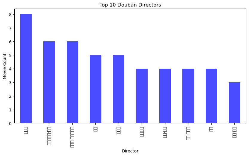
# Top directors by movie count
douban_directors = douban_data['Douban_Info'].str.extract(r'导演: (.+?) ').dropna()
douban_top_directors = douban_directors[0].value_counts().head(10)

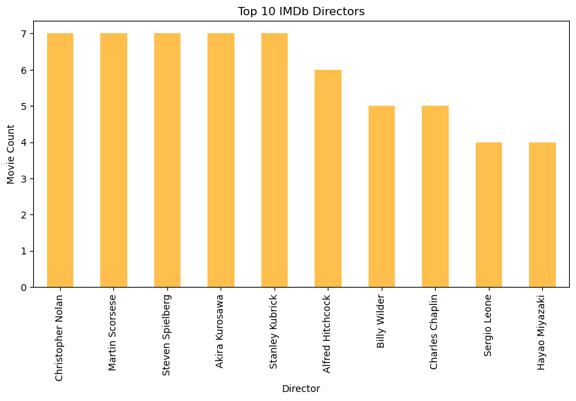
imdb_top_directors = imdb_data['IMDB_Director'].value_counts().head(10)

plt.figure(figsize=(10, 5))
douban_top_directors.plot(kind='bar', alpha=0.7, label='Douban', color='blue')
plt.title('Top 10 Douban Directors')
plt.xlabel('Director')
plt.ylabel('Movie Count')
plt.show()

plt.figure(figsize=(10, 5))
imdb_top_directors.plot(kind='bar', alpha=0.7, label='IMDb', color='orange')
plt.title('Top 10 IMDb Directors')
plt.xlabel('Director')
plt.ylabel('Movie Count')
plt.show()

# Save overlapping movies to a CSV file
overlap_movies.to_csv('overlap_movies.csv', index=False)

# Print results
print(f"豆瓣平均评分: {douban_avg_score}")
print(f"IMDb平均评分: {imdb_avg_score}")
print(f"重叠电影数量: {len(overlap_movies)}")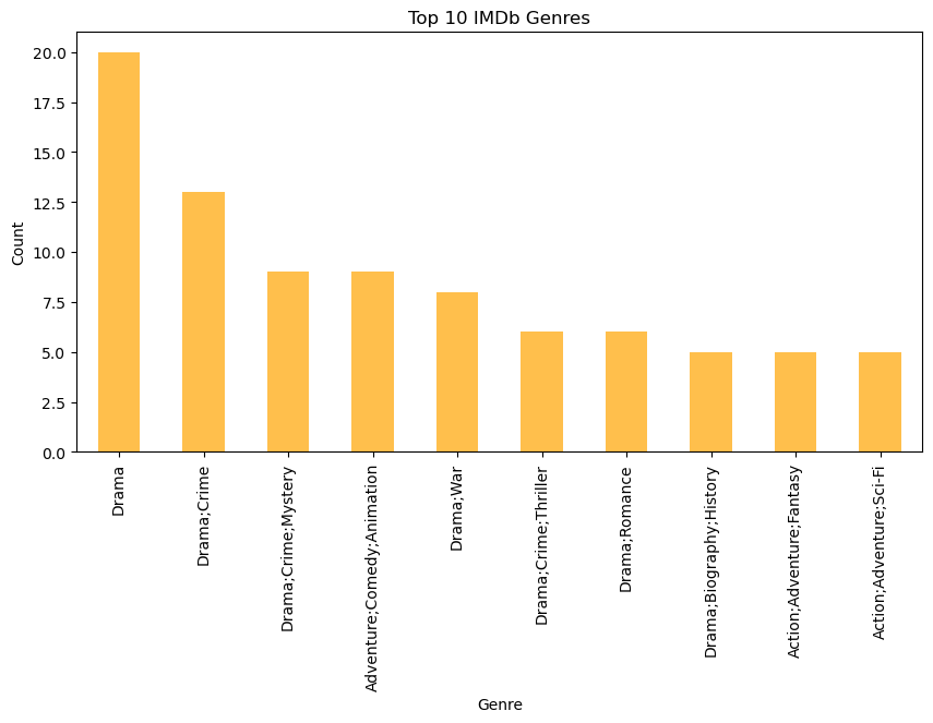

豆瓣平均评分: 8.9396
IMDb平均评分: 8.254
重叠电影数量: 0

Notebooks

Exercises-Chipotle 1

Ex2 - Getting and Knowing your Data

Step 1. Import the necessary libraries

Step 2. Import the dataset from this address.

Step 3. Assign it to a variable called chipo.

Step 4. See the first 10 entries

Step 5. What is the number of observations in the dataset?

Step 6. What is the number of columns in the dataset?

Step 7. Print the name of all the columns.

Step 8. How is the dataset indexed?

Step 9. Which was the most-ordered item?

Step 10. For the most-ordered item, how many items were ordered?

Step 11. What was the most ordered item in the choice_description column?

Step 12. How many items were orderd in total?

Step 13. Turn the item price into a float

Step 13.a. Check the item price type

Step 13.b. Create a lambda function and change the type of item price

Step 2. Import the dataset from this address.

Step 3. Assign it to a variable called chipo.

Step 4. See the first 10 entries

Step 5. Create a histogram of the top 5 items bought

Step 6. Create a scatterplot with the number of items orderered per order price

Hint: Price should be in the X-axis and Items ordered in the Y-axis

Step 7. BONUS: Create a question and a graph to answer your own question.

Exercises-Occupation 1

Ex3 - Getting and Knowing your Data

Step 1. Import the necessary libraries

Step 2. Import the dataset from this address.

Step 3. Assign it to a variable called users and use the ‘user_id’ as index

Step 4. See the first 25 entries

Step 5. See the last 10 entries

Step 6. What is the number of observations in the dataset?

Step 7. What is the number of columns in the dataset?

Step 8. Print the name of all the columns.

Step 9. How is the dataset indexed?

Step 10. What is the data type of each column?

Step 11. Print only the occupation column

Step 12. How many different occupations are in this dataset?

Step 13. What is the most frequent occupation?

Step 14. Summarize the DataFrame.

Step 15. Summarize all the columns

Step 16. Summarize only the occupation column

Step 17. What is the mean age of users?

Step 18. What is the age with least occurrence?

Exercises-World Food Facts 1

Exercise 1

Step 1. Go to https://www.kaggle.com/openfoodfacts/world-food-facts/data

Step 2. Download the dataset to your computer and unzip it.

Step 3. Use the tsv file and assign it to a dataframe called food

Step 4. See the first 5 entries

Step 5. What is the number of observations in the dataset?

Step 6. What is the number of columns in the dataset?

Step 7. Print the name of all the columns.

Step 8. What is the name of 105th column?

Step 9. What is the type of the observations of the 105th column?

Step 10. How is the dataset indexed?

Step 11. What is the product name of the 19th observation?

77fba8e3b056425013930abb11e0a970

4.IMDb and Douban top-250 movie datasets